Appendix. Relaxation times.
A relaxation time is basically the time it takes a decay process to decrease a disturbance. We may look at several different kinds of disturbances and at useful measures of the decay rate. The inverse of the decay rate will be expressed as a time, the relaxation time.
Case (1) A decay of a disturbance with a rate directly proportional to the current size of the disturbance – a first-order decay or first order reaction. Many “disturbances” such as heating an iron rod in air disappear over time, or “relax” toward the earlier state. A simple case is such cooling by convection to air, following Newton’s law. Suppose an iron bar starts out at ambient temperature, Ta. Now heat it to a higher new temperature, T0. The disturbance is the jump in temperature, T’0 = T0 – Ta. We may then watch the decline in temperature as a function of time. In a fairly good approximation, the rate of loss of heat and thus of temperature T at any time, t, is just proportional to the current offset, T’(t) = T(t)-Ta . This is called a linear relaxation process because the rate of change of the variable is linearly proportional to the value of the variable itself. Let ΔT’ be the change in temperature in a short time, Δt. We can take the limit of very short time intervals to use the notation of calculus,
![]()
(This is accurate for a body with rather constant heat capacity at all temperatures). The solution for T’ as a function of time, T’(t), is just the negative exponential,
![]()
Here, e is 2.71828…, the base of the natural logarithms.
This is how T’ looks over time, nice “negative exponential”):
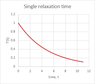
Now to consider this decline as a relaxation process. At very long times the offset decays to zero. The relaxation time, tr, is the time to get to a standard fraction of the original value. An obvious choice is the time when ktr =1, tr=1/k. By that time the disturbance has decayed to a value e-1 = 0.37 or 37% of its initial value. A faster rate, k, gives a shorter relaxation time. We could also use the half-life, the time when e-kt=1/2, which is t1/2=ln(2)/k = 0.693/k. Use whichever one makes you happy.
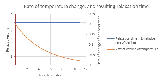
In fact, we can take the “instantaneous” relaxation time. We compute the relative rate of change in the variable at any time: that’s (dT/dt)/T, and let’s give it the opposite sign so it’s a positive value, -(dT/dt)/T. For our example, that is just the value k, at all times. That’s clear from the equation, and it also expresses the constant proportionality between temperature and its rate of decrease. To get a time, we take the inverse of this. When k has the value 0.2, as above, the relaxation time is 1/0.2 = 5.
Case (2) There can be more than one process acting to change a variable – perhaps two ways of cooling, by convection to the air and by radiation. What does the curve look like then? For deviations in temperature that are not too big, say, a 10% increase of absolute temperature (from 20°C = 293K to 322K = 49°C), the cooling by radiation is also a linear process. We then have the equation
![]()
We can rewrite this as
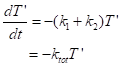
This is still a process with a single relaxation time, tr,net = 1/(k1+k2). Two simultaneous processes acting at the same time look like a single faster process, still linear. The rate is higher and the relaxation time is consequently shorter.
Case (3) A system may have two or more decay processes but showing two or more distinct relaxation times. This can only happen when the second (and third and…) processes get changed in rate from an independent cause. Let’s take two chemical reactions. The first one contributes a rate of change of concentration C of a reactant as
![]()
If the second reaction contributes a change of the same form but with a rate constant k2, we still have only a single relaxation time, tr,net = 1/(k1+k2). However, the rate of reaction of compound C in the second reaction could depend on a second compound, D, that has its own time-dependence:
![]()
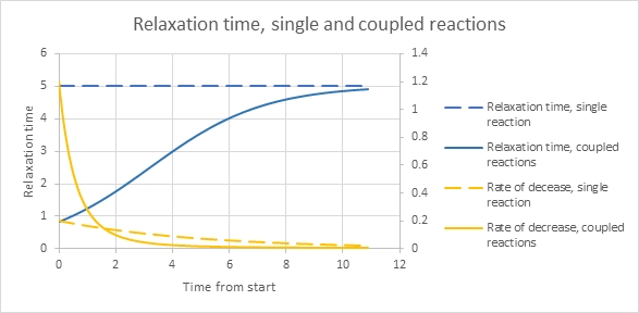
I made a simple model where k1=0.2, k2=0.05 (slower), C at time zero = 1, but D(0) = 20. Then, k2D is 0.05*20 = 1 is bigger than k1 and it dominates the initial rate. I set D to decline fairly quickly as a simple linear rate (negative exponential concentration over time), with a rate constant 0.5. The solid yellow line below shows that there’s a fast initial rate of decrease, knet=k1+k2D with, thus, a short relaxation time. As D declines it progressively loses the ability to affect the rate of decrease to the primary reactant, C. The relative rate of decrease of C stabilizes and we go toward a steady and longer relaxation time appropriate to the reaction of C by itself.
A change of relaxation rate from various causes occurs in the rate of disappearance of CO2 from our atmosphere, if we ever stop pumping in massive amounts! Even while we continue to add much CO2, it’s possible to analyze the changes mathematically to separate out the depletion processes from the addition processes, if not without a lot of work, as has been done). For some disappearance processes such as dissolving CO2 into ocean water, the initial process is linearly dependent on the effective difference in CO2 concentration between air and the sea. It’s also a fair approximation that the rate of uptake of CO2 by land plants starts out as linearly proportional to the increase in CO2. Things get more complicated and then nonlinear as time goes on. The top layer of the ocean gets mixed to various depths as the season changes, mixing low and high CO2 parcels. The plants acclimate their growth to high CO2 and change their rate of growth. They also may run low on some nutrients to support their growth; for others such as nitrogen, they need less of it at high CO2 and can grow better. I’ve done much research on plant responses to high CO2 and I appreciate the complexity. I particularly appreciate the evidence that plants cannot continue to take up 40% of the CO2 we add to the atmosphere. We need to just stop, or even back up and actively remove CO2 from the atmosphere to preserve a livable climate.
Case (4) Of course, a nonlinear decay rate of a single process can look like a change of reaction rate and, thus, a change of relaxation time if we try to view any segment as if it’s a linear reaction rate (any smooth curve over a very short time looks like a straight line, when second derivatives are not important). Here’s the case of a second-order chemical reaction. An example of such a reaction is the dimerization of the compound 2,5-dimethyl-3,4-diphenylcyclopentadienone. Dimerization is just the joining of two molecules into one. The rate of reaction is proportional to the square of the compound’s concentration:
![]()
Obviously the rate slows down as the reaction depletes the concentration. There is a mathematical solution in “closed form,” which is straightforward to derive in calculus,
![]()
Here are the same kinds of plots as for the earlier cases, with arbitrary time units:
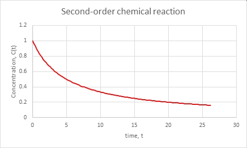
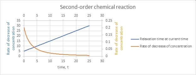
Right, the reaction even as a relative rate gets slower as time goes on and the concentration declines.
Suppose that we didn’t know the nature of the reaction or process going on. We can still do empirical extraction of the relaxation time. We can plot the natural logarithm of the concentration (or relevant variable – temperature, e.g.) and fit a straight line to various sections. For the case above, we have these estimates:
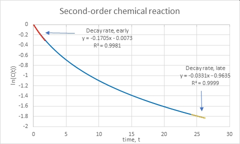
The slope d(ln C)/dt is just (1/C)(dC/dt) and its inverse is the relaxation time at that point. For the beginning of the curve we get the relaxation time τ =1/0.17 = 5.9 and at time t = 25, we get τ=1/0.033=30. Those are close to the analytical results.